Laminar ROI analysis of power in source space

This tutorial demonstrates how to perform laminar inference using an ROI analysis of power in source space, described in [Bonaiuto et al., 2018, Non-invasive laminar inference with MEG: Comparison of methods and source inversion algorithms](https://doi.org/10.1016/j.neuroimage.2017.11.068), and used in [Bonaiuto et al., 2018, Lamina-specific cortical dynamics in human visual and sensorimotor cortices](https://doi.org/10.7554/eLife.33977). A 20Hz oscillation is simulated at a particular cortical location in various layers. Source reconstruction is performed using the Empirical Bayesian Beamformer on the simulated sensor data using a forward model based on a multilayer mesh, thus providing an estimate of source activity on each layer. An ROI is defined by comparing power in the 10-30 Hz frequency band during the time period containing the simulated activity with a prior baseline period at each vertex using paired t-tests. Vertices in either surface with a t-statistic above a percentile threshold of the t-statistics over all vertices in that surface, as well as the corresponding vertices in the other surface, are included in the ROI. This ensures that the contrast used to define the ROI was orthogonal to the subsequent laminar contrast. For each trial, ROI values for each layer are computed by averaging the absolute value of the change in power compared to baseline in that surface within the ROI. Finally, a paired t-test is used to compare the ROI values from each layer over trials. All t-tests are done using corrected noise variance estimates in order to attenuate artifactually high significance values [Ridgway et al., 2012](https://doi.org/10.1016/j.neuroimage.2011.10.027).

Setting up the simulations

Simulations are based on an existing dataset, which is used to define the sampling rate, number of trials, duration of each trial, and the channel layout.

import os
import shutil
import numpy as np
import nibabel as nib
import matplotlib.pyplot as plt
import tempfile

from lameg.invert import invert_ebb, coregister, load_source_time_series
from lameg.laminar import roi_power_comparison
from lameg.simulate import run_current_density_simulation
from lameg.surf import interpolate_data
from lameg.viz import show_surface, color_map
import spm_standalone

# Subject information for data to base the simulations on
subj_id = 'sub-104'
ses_id = 'ses-01'

# Fiducial coil coordinates
nas = [0.9662503311032098, 108.83514306876269, 1.6712361927090313]
lpa = [-74.28671169006893, 20.15061014698176, -29.849056272705948]
rpa = [76.02110531729883, 18.9467849625573, -25.779407159603114]

# Data file to base simulations on
data_file = os.path.join(
    '../test_data',
    subj_id,
    'meg',
    ses_id,
    'spm/spm-converted_autoreject-sub-104-ses-01-001-btn_trial-epo.mat'
)

spm = spm_standalone.initialize()

For source reconstructions, we need an MRI and a surface mesh. The simulations and source reconstructions will be based on a forward model using the multilayer mesh

# Native space MRI to use for coregistration
mri_fname = os.path.join('../test_data', subj_id, 'mri/s2023-02-28_13-33-133958-00001-00224-1.nii' )

# Mesh to use for forward model in the simulations
multilayer_mesh_fname = os.path.join('../test_data', subj_id, 'surf/multilayer.11.ds.link_vector.fixed.gii')

# Load multilayer mesh and compute the number of vertices per layer
mesh = nib.load(multilayer_mesh_fname)
n_layers = 11
verts_per_surf = int(mesh.darrays[0].data.shape[0]/n_layers)

# Inflated meshes for plotting
ds_inflated = nib.load(os.path.join('../test_data', subj_id, 'surf', 'inflated.ds.gii'))
orig_inflated = nib.load(os.path.join('../test_data', subj_id, 'surf', 'inflated.gii'))

We’re going to copy the data file to a temporary directory and direct all output there.

# Extract base name and path of data file
data_path, data_file_name = os.path.split(data_file)
data_base = os.path.splitext(data_file_name)[0]

# Where to put simulated data
tmp_dir = tempfile.mkdtemp()

# Copy data files to tmp directory
shutil.copy(
    os.path.join(data_path, f'{data_base}.mat'),
    os.path.join(tmp_dir, f'{data_base}.mat')
)
shutil.copy(
    os.path.join(data_path, f'{data_base}.dat'),
    os.path.join(tmp_dir, f'{data_base}.dat')
)

# Construct base file name for simulations
base_fname = os.path.join(tmp_dir, f'{data_base}.mat')

Invert the subject’s data using the multilayer mesh. This step only has to be done once - this is just to compute the forward model that will be used in the simulations

# Patch size to use for inversion (in this case it matches the simulated patch size)
patch_size = 5
# Number of temporal modes to use for EBB inversion
n_temp_modes = 4

# Coregister data to multilayer mesh
coregister(
    nas,
    lpa,
    rpa,
    mri_fname,
    multilayer_mesh_fname,
    base_fname,
    spm_instance=spm
)

# Run inversion
[_,_] = invert_ebb(
    multilayer_mesh_fname,
    base_fname,
    n_layers,
    patch_size=patch_size,
    n_temp_modes=n_temp_modes,
    spm_instance=spm
)

Simulating a signal on the pial surface

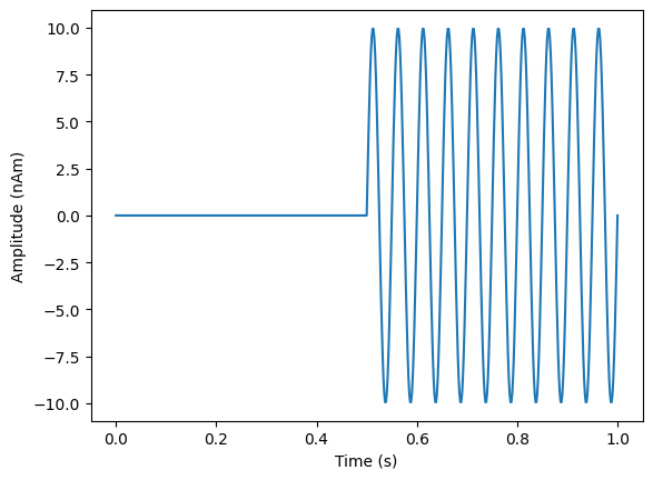
We’re going to simulate 1s of signal with a 20Hz sine wave that starts at 0.5s with a dipole moment of 10nAm

# Frequency of simulated sinusoid (Hz)
freq = 20
# Strength of simulated activity (nAm)
dipole_moment = 10
# Sampling rate (must match the data file)
s_rate = 600

# Generate 1s of a sine wave at a sampling rate of 600Hz (to match the data file)
time = np.linspace(0,1,s_rate+1)
sim_signal = np.zeros(time.shape).reshape(1,-1)
t_idx=np.where(time>=0.5)[0]
sim_signal[0,t_idx] = np.sin(time[t_idx]*freq*2*np.pi)

plt.plot(time,dipole_moment*sim_signal[0,:])
plt.xlabel('Time (s)')
plt.ylabel('Amplitude (nAm)')

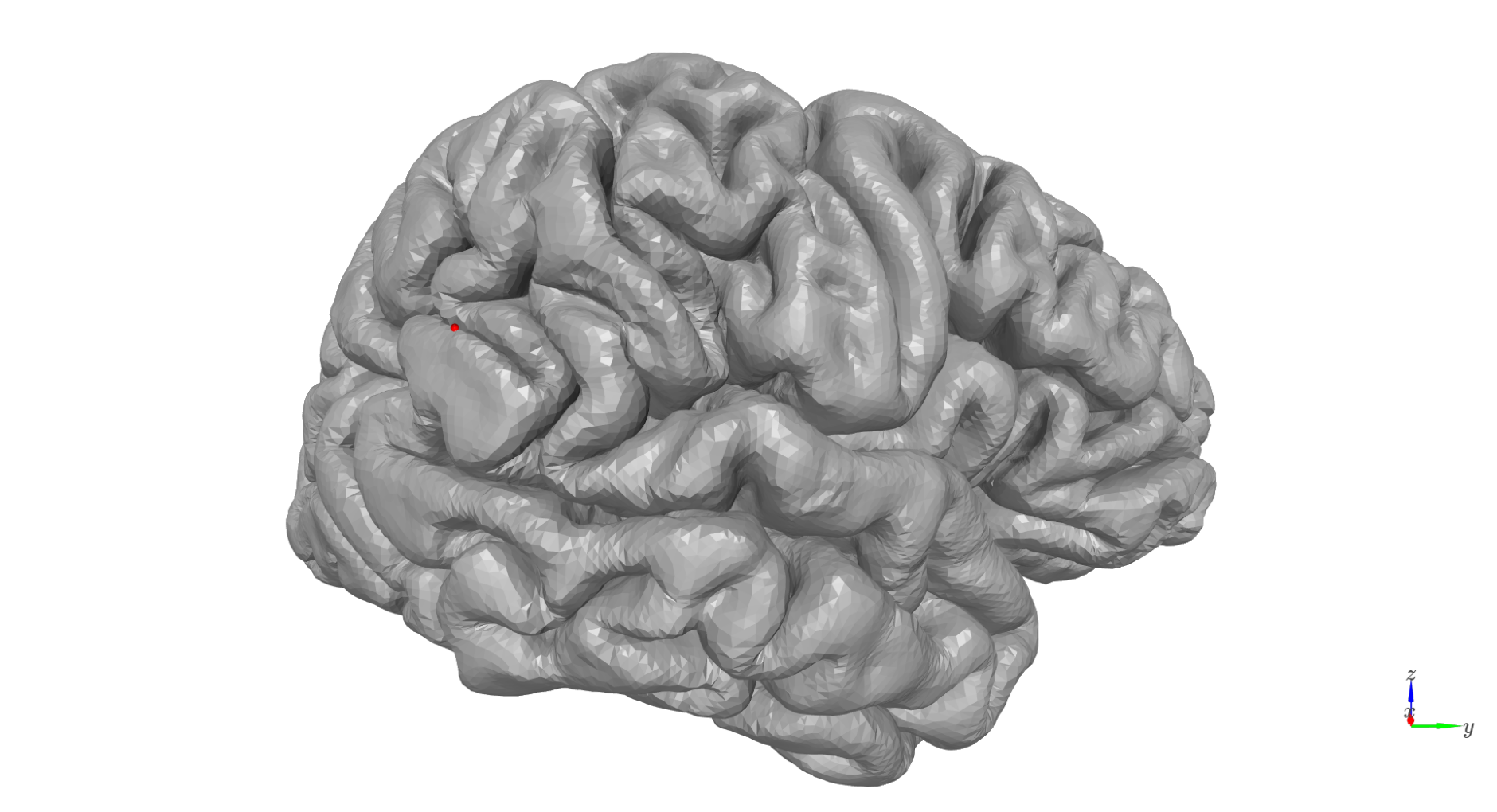
We need to pick a location (mesh vertex) to simulate at

# Vertex to simulate activity at
sim_vertex=24585

pial_ds_mesh_fname = os.path.join('../test_data', subj_id, 'surf', 'pial.ds.link_vector.fixed.gii')
pial_ds_mesh = nib.load(pial_ds_mesh_fname)
pial_coord = pial_ds_mesh.darrays[0].data[sim_vertex,:]
pial_mesh_fname = os.path.join('../test_data', subj_id, 'surf', 'pial.gii')
pial_mesh = nib.load(pial_mesh_fname)
cam_view = [152, 28, 15,
            3.5, 26, 38.5,
            0, 0, 1]
plot = show_surface(
    pial_mesh,
    opacity=1,
    coords=pial_coord,
    coord_size=2,
    camera_view=cam_view
)

We’ll simulate a 5mm patch of activity with -5 dB SNR at the sensor level. The desired level of SNR is achieved by adding white noise to the projected sensor signals

# Simulate at a vertex on the pial surface
pial_vertex = sim_vertex
prefix = f'sim_{sim_vertex}_pial_'

# Size of simulated patch of activity (mm)
sim_patch_size = 5
# SNR of simulated data (dB)
SNR = -10

# Generate simulated data
pial_sim_fname = run_current_density_simulation(
    base_fname,
    prefix,
    pial_vertex,
    sim_signal,
    dipole_moment,
    sim_patch_size,
    SNR,
    spm_instance=spm
)

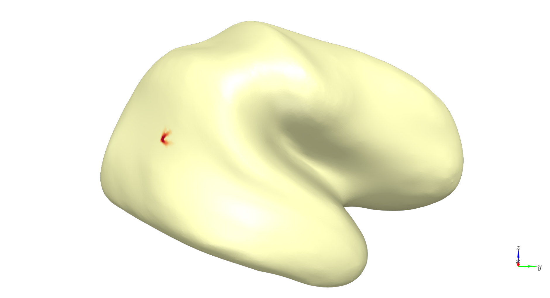
Laminar comparison (pial - white matter)

Now we can run source reconstruction using a source model based on the multi-laminar surface, define an ROI based on the change in power from a baseline time period, and then compare the change in power between the pial and white matter surfaces. First we’ll run the inversion.

# Coregister data to multilayer mesh
coregister(
    nas,
    lpa,
    rpa,
    mri_fname,
    multilayer_mesh_fname,
    pial_sim_fname,
    spm_instance=spm
)

# Run inversion on simulated data in a 5Hz window around the simulated frequency using the multilayer surface
[_,_,MU] = invert_ebb(
    multilayer_mesh_fname,
    pial_sim_fname,
    n_layers,
    foi=[freq-10, freq+10],
    patch_size=patch_size,
    n_temp_modes=n_temp_modes,
    return_mu_matrix=True,
    spm_instance=spm
)

Now we can defined the ROI based on where the change in power from baseline exceeds some percentile threshold in either the pial or the white matter surface, then average the change in power within the ROI, and compare the magnitude of the change between layers. The t-statistic here should be positive, indicating a greater change in power from baseline in the pial surface, because we simulated activity on the pial surface

laminar_t_statistic, laminar_p_value, df, roi_idx = roi_power_comparison(
    pial_sim_fname,
    [0, 500],
    [-500, 0],
    mesh,
    n_layers,
    99.99,
    mu_matrix=MU
)
print(f't({df})={laminar_t_statistic}, p={laminar_p_value}')

roi=np.zeros(verts_per_surf)
roi[roi_idx]=1

# Interpolate for display on the original inflated surface
interpolated_data = interpolate_data(orig_inflated, ds_inflated, roi)

# Plot colors and camera view
c_range = [-1, 1]
cam_view=[289, 32, -19,
          3.5, 29, 26,
          0, 0, 1]

# Plot change in power on each surface
colors,_ = color_map(
    interpolated_data,
    "RdYlBu_r",
    c_range[0],
    c_range[1]
)
plot = show_surface(orig_inflated, vertex_colors=colors, info=True, camera_view=cam_view)

White matter surface simulation with pial - white matter ROI comparison

Let’s simulate the same pattern of activity, in the same location, but on the white matter surface. This time, there should be a greater change in power on the white matter surface.

# Simulate at the corresponding vertex on the white matter surface
white_vertex = (n_layers-1)*verts_per_surf+sim_vertex
prefix = f'sim_{sim_vertex}_white_'

# Generate simulated data
white_sim_fname = run_current_density_simulation(
    base_fname,
    prefix,
    white_vertex,
    sim_signal,
    dipole_moment,
    sim_patch_size,
    SNR,
    spm_instance=spm
)

# Coregister data to multilayer mesh
coregister(
    nas,
    lpa,
    rpa,
    mri_fname,
    multilayer_mesh_fname,
    white_sim_fname,
    spm_instance=spm
)

# Run inversion on simulated data in a 5Hz window around the simulated frequency using the multilayer surface
[_,_,MU] = invert_ebb(
    multilayer_mesh_fname,
    white_sim_fname,
    n_layers,
    foi=[freq-10, freq+10],
    patch_size=patch_size,
    n_temp_modes=n_temp_modes,
    return_mu_matrix=True,
    spm_instance=spm
)

# Compare power t statistic should be negative (more power in white matter layer)
laminar_t_statistic, laminar_p_value, df, roi_idx = roi_power_comparison(
    white_sim_fname,
    [0, 500],
    [-500, 0],
    mesh,
    n_layers,
    99.99,
    mu_matrix=MU
)
print(f't({df})={laminar_t_statistic}, p={laminar_p_value}')

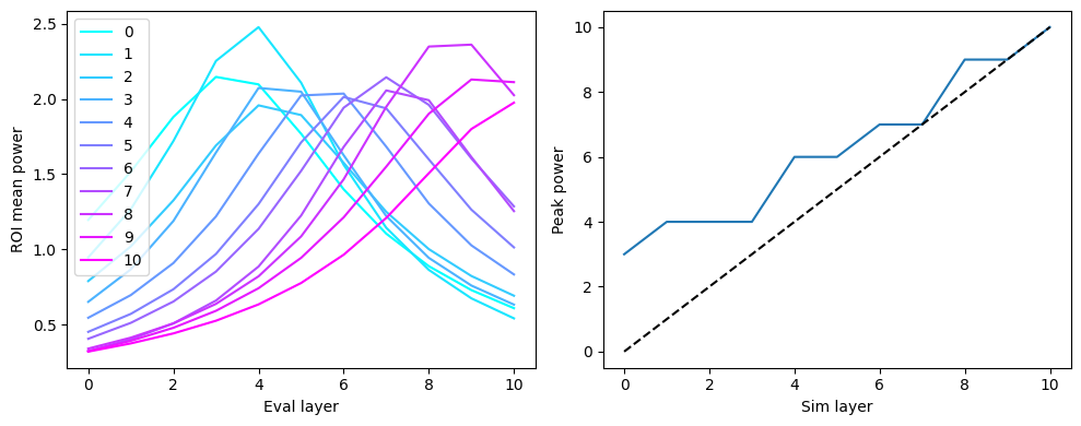
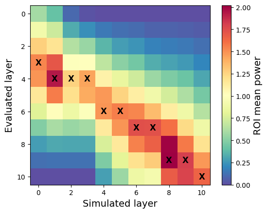
Simulation in each layer with ROI power analysis across layers

That was the ROI analysis with two surfaces: the white matter and pial surfaces. Let’s now simulate on each layer, and for each simulation, look at the change in power from baseline within the ROI across all layers. We’ll turn off SPM visualization here.

# Now simulate at the corresponding vertex on each layer, and for each simulation, compute power in
# all layers
all_layerPow=[]

for sl in range(n_layers):
    print(f'Simulating in layer {sl}')
    l_vertex = sl*verts_per_surf+sim_vertex
    prefix = f'sim_{sim_vertex}_{sl}_'

    l_sim_fname = run_current_density_simulation(
        base_fname,
        prefix,
        l_vertex,
        sim_signal,
        dipole_moment,
        sim_patch_size,
        SNR,
        spm_instance=spm
    )

    coregister(
        nas,
        lpa,
        rpa,
        mri_fname,
        multilayer_mesh_fname,
        l_sim_fname,
        viz=False,
        spm_instance=spm
    )

    [_,_,MU] = invert_ebb(
        multilayer_mesh_fname,
        l_sim_fname,
        n_layers,
        foi=[freq-10, freq+10],
        patch_size=patch_size,
        n_temp_modes=n_temp_modes,
        return_mu_matrix=True,
        viz=False,
        spm_instance=spm
    )

    laminar_t_statistic, laminar_p_value, df, roi_idx = roi_power_comparison(
        l_sim_fname,
        [0, 500],
        [-500, 0],
        mesh,
        n_layers,
        99.99,
        mu_matrix=MU
    )

    roi_pow=[]
    for il in range(n_layers):
        layer_roi_verts = il*verts_per_surf+roi_idx
        layer_ts, time, _ = load_source_time_series(
            l_sim_fname,
            mu_matrix=MU,
            vertices=layer_roi_verts.astype(int)
        )
        # Compute power in baseline and stimulus time periods
        base_t_idx = np.where(time<0)[0]
        exp_t_idx = np.where(time>=0)[0]

        layer_base_power = np.squeeze(np.var(layer_ts[:,base_t_idx,:],axis=1))
        layer_exp_power = np.squeeze(np.var(layer_ts[:,exp_t_idx,:],axis=1))
        layer_power_change = (layer_exp_power-layer_base_power)/layer_base_power

        roi_pow.append(np.abs(np.mean(layer_power_change,axis=0)))

    all_layerPow.append(roi_pow)
all_layerPow=np.array(all_layerPow)

# Average power over trials
mean_layerPow=np.mean(all_layerPow,axis=-1)

col_r = plt.cm.cool(np.linspace(0,1, num=n_layers))
plt.figure(figsize=(10,4))

# For each simulation, plot the power in each layer model
plt.subplot(1,2,1)
for l in range(n_layers):
    layerPow=mean_layerPow[l,:]
    plt.plot(layerPow, label=f'{l}', color=col_r[l,:])
plt.legend()
plt.xlabel('Eval layer')
plt.ylabel('ROI mean power')

# For each simulation, find which layer had the greatest power
plt.subplot(1,2,2)
peaks=[]
for l in range(n_layers):
    layerPow=mean_layerPow[l,:]
    pk=np.argmax(layerPow)
    peaks.append(pk)
plt.plot(peaks)
plt.xlim([-0.5,10.5])
plt.ylim([-0.5,10.5])
plt.plot([0,10],[0,10],'k--')
plt.xlabel('Sim layer')
plt.ylabel('Peak power')
plt.tight_layout()
plt.savefig('roi_power.pdf')

mean_layerPow=np.mean(all_layerPow,axis=-1)

# Normalization step
norm_mean_layerPow = np.zeros(mean_layerPow.shape)
for l in range(n_layers):
    norm_mean_layerPow[l,:] = mean_layerPow[l,:] - np.min(mean_layerPow[l,:])

# Transpose for visualization
im=plt.imshow(norm_mean_layerPow.T, cmap='Spectral_r')

# Find the indices of the max value in each column
max_indices = np.argmax(norm_mean_layerPow, axis=1)

# Plot an 'X' at the center of the square for each column's maximum
for idx, max_idx in enumerate(max_indices):
    plt.text(idx, max_idx, 'X', fontsize=12, ha='center', va='center', color='black', weight='bold')

plt.xlabel('Simulated layer', fontsize=14)
plt.ylabel('Evaluated layer', fontsize=14)
cb=plt.colorbar(im)
cb.set_label('ROI mean power', fontsize=14)
plt.savefig('roi_power_matrix.pdf')

spm.terminate()

# Delete simulation files
shutil.rmtree(tmp_dir)